Assignment样板：两篇Coursework范例

a. For the general data set:
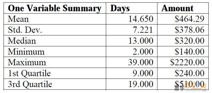
One Variable Summary Days Amount
Mean 14.650 $464.29
Std. Dev. 7.221 $378.06
Median 13.000 $320.00
Minimum 2.000 $140.00
Maximum 39.000 $2220.00
1st Quartile 9.000 $240.00
3rd Quartile 19.000 $510.00
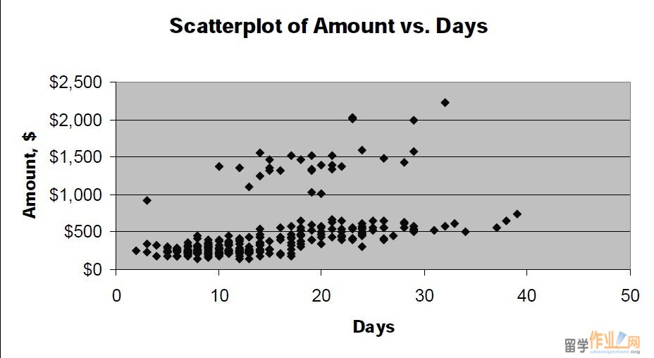
Scatterplot of Amount vs. Days
$0
$500
$1,000
$1,500
$2,000
$2,500
0 10 20 30 40 50
Days
Amount, $
The number of days ranges from 2 to 39. On average, 14.65 days have passed since
assignment 格式r was billed. 50% of the customers were billed less than 13 days ago.
Amount of debt is within the range from $140 to $2,220. On average, a customer
owes $464.29. 50% of the customers owe less than $320.
Correlation coefficient equals to 0.489 and indicates moderate positive relationship.
However, this number should be treated very carefully as the scatterplot indicates presence of
two distinct populations within the group. It is advisable to divide the customers into two
groups based on the amount they owe.
b. Two groups are introduced for further analysis: Small debtors – customers who owe
between $0 and $900 and Big debtors – customers who owe more $900.
The pivot table indicates that average of Days for Big debtors is significantly higher
than for Small debtors.

 

Coursework 2
Average of Days Days
Amount 0-19 20-40 Grand Total
140-900 11.0 25.3 14.1
>900 14.9 24.2 19.2
Grand Total 11.3 25.0 14.7
For Small Debtors (250 customer owing in total $86,370):
One Variable Summary Days Amount

http://www.uka
 

 

Mean 14.100 $345.48
Variance 51.135 17819.25
Std. Dev. 7.151 $133.49
Median 12.000 $300.00#p#分页标题#e#
Minimum 2.000 $140.00
Maximum 39.000 $750.00
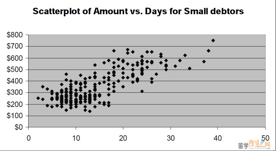
Scatterplot of Amount vs. Days for Small debtors
$0
$100
$200
$300
$400
$500
$600
$700
$800
0 10 20 30 40 50
Correlation 0.780 indicates strong positive relationship.
For Big debtors (30 customer owing in total $43,630):
One Variable Summary Days Amount
Mean 19.233 $1454.33
Variance 38.323 86370.23
Std. Dev. 6.191 $293.89
Median 19.000 $1390.00
Minimum 3.000 $930.00
Maximum 32.000 $2220.00
Coursework 3
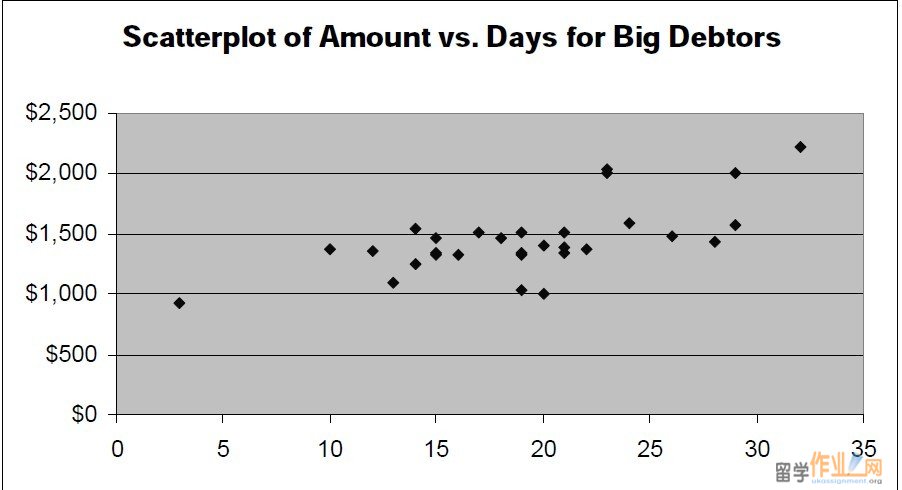
Scatterplot of Amount vs. Days for Big Debtors
$0
$500
$1,000
$1,500
$2,000
$2,500
0 5 10 15 20 25 30 35
Correlation 0.655 – moderate positive relationship.

 

c. As recently the company has faced a worrying situation with accounts receivable we
have conducted the analysis of our customer base with regard to amount owed currently and
number of days that has passed since the customer was billed.
If all the customers were exactly the same each customer would owe $464.29 and
would have been billed 14.65 days ago (the mean numbers for general group). However, the
two distinct groups in the set can be seen and, for purpose of better analysis, we have
separated the data into Small debtors (250 customers owing in total $86,370) and Big debtors
(30 customer owing in total $43,630).
This division resulted in significant increase in correlation coefficient for both groups
in comparison to the general population. Correlation coefficient values (0.780 and 0.655)
indicate strong positive relationship between amount of debt and number of days. That means
that customers who receive bigger amount of credit tend to pay later compared to the group’s
average. An average big debtor pays back later than the average small debtor (19.2 vs. 14.1
days on average).
It is recommended:
§ To implement stricter credit policy and receivables collection for high amounts
of credit for each group separately (e.g. more than $500 for small debtors and
more than $1,500 for big debtors);
Coursework 4
§ To concentrate on big debtors as, on average, they pay later and own
significant amounts (less than 11% of customers owe 33.6% of the total
amount of receivables).
3. ‘All-For-Kids’:
i. Storage costs: one pack gets allocated the cost of renting 1.5/15 = 0.1 feet (£10)
Let S be average stock throughout the year. Then annual holding stock cost is:
0.15*£2.50*365*S + £10*S = £146.9*S
Storage cost constitutes 10S/146.9S = 6.8% out of total holding stock cost.#p#分页标题#e#
ii. The quantity ordered should equal to 2S. With the optimal order schedule the cost of orderhandling
and shipment would offset the cost of holding one more additional day of stock:
0.15*2.50*S + (10/365)*S = 30
Solving we find S = 75.
The optimal order should be 2S = 150 packs and made every three working days.
iii. It has been assumed that when the new order is delivered the actual quantity on stock is
zero. It is not very realistic with regard to real businesses because of demand fluctuations and
safety stock that is usually kept.
iv. The annual number of orders placed by one store: (300*52)/150 = 104
The annual number of orders placed by all stores: 104*120 = 12,480
Annual savings: 12, 480*£10 = £124, 800.
As the cost of the equipment is £120,000 the payback period is less than a year and it is
recommended to buy the equipment.
v. If the manager chooses to increase the quantity ordered it would result in savings coming
from discounts and decrease in order-handling fees as well as in increasing costs from
holding extra stock.
If the new quantity is 500, the savings would be 500*£0.05 + (500/150-1)*30 = £95
The order cycle increases by (500 – 150)/(300/6) = 4 days
Coursework 5
The additional costs are 0.15*2.50*500/2*4 + (10/365)*500/2*4 = £ 375.
Conducting the similar analysis for lower limit of every range, we see that in all cases
additional costs are higher than additional savings and the store’s manager should keep the
order level at 150 packs.